Dr. Javier Quilez Oliete, an experienced freelance bioinformatics consultant on Kolabtree, provides a comprehensive guide to DNA sequencing data analysis, including tools and software used to read data.
Introduction
Deoxyribonucleic acid (DNA) is the molecule that carries most of the genetic information of an organism. (In some types of virus, genetic information is carried by ribonucleic acid (RNA).) Nucleotides (conventionally represented by the letters A, C, G or T) are the basic units of DNA molecules. Conceptually, DNA sequencing is the process of reading the nucleotides that comprise a DNA molecule (e.g. “GCAAACCAAT” is a 10-nucleotide DNA string). Current sequencing technologies produce millions of such DNA reads in a reasonable time and at a relatively low cost. As a reference, the cost of sequencing a human genome – a genome is the complete set of DNA molecules in an organism – has dropped the $100 barrier and it can be done in a matter of days. This contrasts with the first initiative to sequence the human genome, which was completed in a decade and had a cost of about $2.7 billions.
This capability to sequence DNA at high throughput and low cost has enabled the development of a growing number of sequencing-based methods and applications. For example, sequencing entire genomes or their protein-coding regions (two approaches known respectively as whole genome and exome sequencing) in disease and healthy individuals can hint to disease-causing DNA alterations. Also, the sequencing of the RNA that is transcribed from DNA—a technique known as RNA-sequencing—is used to quantify gene activity and how this changes in different conditions (e.g. untreated versus treatment). On the other side, chromosome conformation capture sequencing methods detect interactions between nearby DNA molecules and thus help to determine the spatial distribution of chromosomes within the cell.
Common to these and other applications of DNA sequencing is the generation of datasets in the order of the gigabytes and comprising millions of read sequences. Therefore, making sense of high-throughput sequencing (HTS) experiments requires substantial data analysis capabilities. Fortunately, dedicated computational and statistical tools and relatively standard analysis workflows exist for most HTS data types. While some of the (initial) analysis steps are common to most sequencing data types, more downstream analysis will depend on the kind of data and/or the ultimate goal of the analysis. Below I provide a primer on the fundamental steps in the analysis of HTS data and I refer to popular tools.
Some of the sections below are focused on the analysis of data generated from short-read sequencing technologies (mostly Illumina), as these have historically dominated the HTS market. However, newer technologies that generate longer reads (e.g. Oxford Nanopore Technologies, PacBio) are gaining ground rapidly. As long-read sequencing has some particularities (e.g. higher error-rates), specific tools are being developed for the analysis of this sort of data.
Quality control (QC) of raw reads
The eager analyst will start the analysis from FASTQ files; the FASTQ format has for long been the standard to store short-read sequencing data. In essence, FASTQ files contain the nucleotide sequence and the per-base calling quality for millions of reads. Although file size will depend on the actual number of reads, FASTQ files are typically large (in the order of megabytes and gigabytes) and compressed. Of note, most tools that use FASTQ files as input can handle them in compressed format so, in order to save disk space, it is recommended not to uncompress them. As a convention, here I will equate a FASTQ file to a sequencing sample.
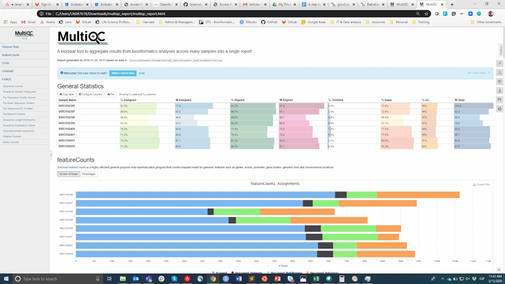
FastQC is likely the most popular tool to carry out the QC of the raw reads. It can be run through a visual interface or programmatically. While the first option may be more convenient for users who do not feel comfortable with the command-line environment, the latter offers incomparable scalability and reproducibility (think of how tedious and error-prone it can be to manually run the tool for tens of files). Either way, the main output of FastQC is an HTML file reporting key summary statistics about the overall quality of the raw sequencing reads from a given sample. Inspecting tens of FastQC reports one by one is tedious and it complicates the comparison across samples. Therefore, you may want to use MultiQC, which aggregates the HTML reports from FastQC (as well as from other tools used downstream, e.g. adapter trimming, alignment) into a single report.

MultiQC
QC information is intended to allow the user to judge whether samples have good quality and can be therefore used for the subsequent steps or they need to be discarded. Unfortunately, there is not a consensus threshold based on the FastQC metrics to classify samples as of good or bad quality. The approach that I use is the following. I expect all samples that have gone through the same procedure (e.g. DNA extraction, library preparation) to have similar quality statistics and a majority of “pass” flags. If some samples have lower-than-average quality, I will still use them in the downstream analysis bearing this in mind. On the other side, if all samples in the experiment systematically get “warning” or “fail” flags in multiple metrics (see this example), I suspect that something went wrong in the experiment (e.g. bad DNA quality, library preparation, etc.) and I recommend repeating it.
Read trimming
QC of raw reads helps to identify problematic samples but it does not improve the actual quality of the reads. To do so, we need to trim reads to remove technical sequences and low-quality ends.
Technical sequences are leftovers from the experimental procedure (e.g. sequencing adapters). If such sequences are adjacent to the true sequence of the read, alignment (see below) may map reads to the wrong position in the genome or decrease the confidence in a given alignment. Besides technical sequences, we may also want to remove sequences of biological origin if these are highly present among the reads. For instance, suboptimal DNA preparation procedures may leave a high proportion of DNA-converted ribosomal RNA (rRNA) in the sample. Unless this type nucleic acid is the target of the sequencing experiment, keeping reads derived from rRNA will just increase the computational burden of the downstream steps and may confound the results. Of note, if the levels of technical sequences, rRNA or other contaminant are very high, which will probably have been already highlighted by the QC, you may want to discard the whole sequencing sample.
In short-read sequencing, the DNA sequence is determined one nucleotide at a time (technically, one nucleotide every sequencing cycle). In other words, the number of sequencing cycles determines read length. A known issue of HTS sequencing methods is the decay of the accuracy with which nucleotides are determined as sequencing cycles accumulate. This is reflected in an overall decrease of the per-base calling quality especially towards the end of the read. As happens with technical sequences, trying to align reads that contain low-quality ends can lead to misplacement or poor mapping quality.
To remove technical/contaminant sequences and low-quality ends, read trimming tools like Trimmomatic and Cutadapt exist and are widely used. In essence, such tools will remove technical sequences (internally available and/or provided by the user) and trim reads based on quality while maximizing read length. Reads that are left too short after the trimming are discarded (reads excessively short, e.g. <36 nucleotides, complicate the alignment step as these will likely map to multiple sites in the genome). You may want to look at the percentage of reads that survive the trimming, as a high-rate of discarded reads is likely a sign of bad-quality data.
Finally, I typically re-run FastQC on the trimmed reads to check that this step was effective and systematically improved the QC metrics.
Alignment
With exceptions (e.g de novo assembly), alignment (also referred to as mapping) is typically the next step for most HTS data types and applications. Read alignment consists in determining the position in the genome from which the sequence of the read derived (typically expressed as chromosome:start-end). Hence, at this step we require the use of a reference sequence to align/map the reads on.
The choice of the reference sequence will be determined by multiple factors. For one, the species from which the sequenced DNA is derived. While the number of species with a high-quality reference sequence available is increasing, this may be still not the case for some less studied organisms. In those cases, you may want to align reads to a evolutively close species for which a reference genome is available. For instance, as there is not a reference sequence for the genome of the coyote, we can use that of the closely related dog for the read alignment. Similarly, we may still want to align our reads to a closely related species for which a higher-quality reference sequence exists. For example, while the genome of the gibbon has been published, this is broken into thousands of fragments that do not fully recapitulate the organization of that genome into tens of chromosomes; in that case, carrying out the alignment using the human reference sequence may be beneficial.
Another factor to consider is the version of the reference sequence assembly, since new versions are released as the sequence is updated and improved. Importantly, the coordinates of a given alignment can vary between versions. For instance, multiple versions of the human genome can be found in the UCSC Genome Browser. In any species, I strongly favor migrating to the newest assembly version once that is fully released. This may cause some nuisance during the transition, as already existing results will be relative to older versions, but it pays off in the long run.
Besides, the type of sequencing data also matters. Reads generated from DNA-seq, ChIP-seq or Hi-C protocols will be aligned to the genome reference sequence. On the other side, as RNA transcribed from DNA is further processed into mRNA (i.e. introns removed), many RNA-seq reads will fail to align to a genome reference sequence. Instead, we need to either align them to transcriptome reference sequences or use split-aware aligners (see below) when using the genome sequence as a reference. Related to this is the choice of source for the annotation of the reference sequence, that is, the database with the coordinates of the genes, transcripts, centromeres, etc. I typically use the GENCODE annotation as it combines comprehensive gene annotation and transcript sequences.
A long list of short-read sequence alignment tools have been developed (see the Short-read sequence alignment section here). Reviewing them is beyond the scope of this article (details about the algorithms behind these tools can be found here). In my experience, among the most populars are Bowtie2, BWA, HISAT2, Minimap2, STAR and TopHat. My recommendation is that you choose your aligner based considering key factors like the type of HTS data and application as well as acceptance by the community, quality of the documentation and number of users. E.g. one needs aligners like STAR or Bowtie2 that are aware of exon-exon junctions when mapping RNA-seq to the genome.
Common to most mappers is the need to index the sequence used as reference before the actual alignment takes place. This step may be time consuming but it only needs to be done once for each reference sequence. Most mappers will store alignments in SAM/BAM files, which follow the SAM/BAM format (BAM files are binary versions of SAM files). The alignment is among the most computation and time consuming steps in the analysis of sequencing data and SAM/BAM files are heavy (in the order of gigabytes). Therefore, it is important to make sure that you have the required resources (see the final section below) to run the alignment in a reasonable time and store the results. Similarly, due to the size and binary format of BAM files, avoid opening them with text editors; instead use Unix commands or dedicated tools like SAMtools.
From the alignments
I would say that there is not a clear common step after the alignment, since at this point is where each HTS data type and application may differ.
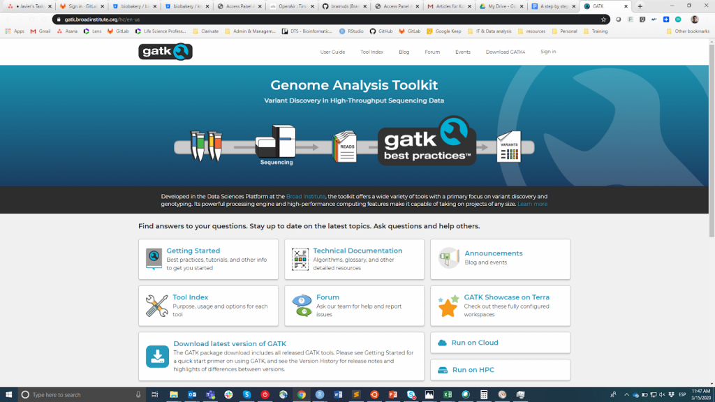
A common downstream analysis for DNA-seq data is variant calling, that is, the identification of positions in the genome that vary relative to the genome reference and between individuals. A popular analysis framework for this application is GATK for single nucleotide polymorphism (SNP) or small insertions/deletions (indels) (Figure 2). Variants comprising larger chunks of DNA (also referred to as structural variants) require dedicated calling methods (see this article for a comprehensive comparison). As with the aligners, I advise selecting the right tool considering key factors like the sort of variants (SNP, indel or structural variants), acceptance by the community, quality of the documentation and number of users.

Probably the most frequent application of RNA-seq is gene expression quantification. Historically, reads needed to be aligned to the reference sequence and then the number of reads aligned to a given gene or transcript was used as a proxy to quantify its expression levels. This alignment+quantification approach is performed by tools like Cufflinks, RSEM or featureCounts. However, scuh approach has been increasingly surpassed by newer methods implemented in software like Kallisto and Salmon. Conceptually, with such tools the full sequence of a read does not need to be aligned to the reference sequence. Instead, we only need to align enough nucleotides to be confident that a read originated from a given transcript. Put it simply, the alignment+quantification approach is reduced to a single step. This approach is known as pseudo-mapping and greatly increases the speed of the gene expression quantification. On the other side, keep in mind that pseudo-mapping will not be suitable for applications where the full alignment is needed (e.g. variant calling from RNA-seq data).
Another example of the differences in the downstream analysis steps and the required tools across sequencing-based application is ChIP-seq. Reads generated with such technique will be used for peak calling, which consists in detecting regions in the genome with a significant excess of reads that indicates where the target protein is bound. Several peak callers exist and this publication surveys them. As a final example I will mention Hi-C data, in which alignments are used as input for tools that determine the interaction matrices and, from these, the 3D-features of the genome. Commenting on all the sequencing-based assays beyond the scope of this article (for a relatively complete list see this article).
Before you start…
The remaining part of this article touches on aspects that may be not strictly considered as steps in the analysis of HTS data and that are largely ignored. In contrast, I argue that it is capital that you think about the questions posed in Table 1 before you start analyzing HTS data (or any kind of data indeed), and I have written on these topics here and here.
Table 1
| Think about it | Proposed action |
| Do you have all the information of your sample needed for the analysis? | Collect systematically the metadata of the experiments |
| Will you be able to identify unequivocally your sample? | Establish a system to assign each sample a unique identifier |
| Where will data and results be? | Structured and hierarchical organization of the data |
| Will you be able to process multiple samples seamlessly? | Scalability, parallelization, automatic configuration and modularity of the code |
| Will you or anybody else be able to reproduce the results? | Document your code and procedures! |
As mentioned above, HTS raw data and some of the files generated during their analysis are in the order of gigabytes, so it is not exceptional that a project including tens of samples requires terabytes of storage. Besides, some steps in the analysis of HTS data are computationally intensive (e.g. alignment). However, the storage and computing infrastructure required for analyzing HTS data is an important consideration and it is often overlooked or not discussed. As an example, as part of a recent analysis, we reviewed tens of published papers performing phenome-wide association analysis (PheWAS). Modern PheWAS analyze 100-1,000s of both genetic variants and phenotypes, which results in important data storage and computing power. And yet, virtually none of the papers we reviewed commented on the infrastructure needed for the PheWAS analysis. Not surprisingly, my recommendation is that you plan upfront the storage and computing requirements that you will face and share them with the community.
Need help with analyzing DNA sequencing data? Get in touch with freelance bioinformatics specialist and genomics experts on Kolabtree.


